Pre-training Large Language Models at Scale
Language modeling is a key component of modern NLP systems. In the simplest sense, a language model is a probability distribution over the words in a language, i.e. it captures the semantic context of the language’s vocabulary. With a good model of a given language, we can achieve a high performance on many downstream NLP tasks like speech processing, reading comprehension, machine translation, and so on. The caveat, however, is that languages are complex, and to adequately capture the intricacies of a language, we need to learn the right semantic context of the entire (or relevant subset of) vocabulary by learning from many numerous varying examples — which gives rise to the notion of Large Language Models (LLM).
How are Large Language Models (LLMs) used?
____
Large Language Models (LLMs) are typically pre-trained on a large set of data from general sources (wikipedia, blogs, academic journals, etc.) and are later fine-tuned on a downstream task; the model gains an abstract understanding of the language in the pre-training step and is then updated to provide a more specific output prediction for the desired NLP task. The benefit of this two-staged approach (Figure 1) is that the pre-training step is significantly more computationally expensive than fine-tuning but it only needs to be done once. The same pre-trained model can then be fine-tuned for a variety of different applications.

Another important benefit of LLMs is that the data used to pre-train the model does not need to be labeled (since we are simply learning the rules of the language and not trying to perform any specific task). This enables our model to learn from larger amounts of data and, thereby, perform significantly better than a model trained only on a limited set of labeled examples.
In the next section, we briefly describe the architecture of one of the most popular LLM in recent years, i.e. the BERT model. Note: Readers are expected to have a basic understanding of the BERT model; the purpose of the following section is simply to provide a high level review of the architecture and hyperparameters of the model which is necessary to understand the scaling issue of LLMs.
The BERT Architecture
____
BERT — which stands for Bidirectional Encoder Representations from Transformers — is a LLM developed by the researchers at Google [Devlin et al.]2. The BERT model is based on the concept of Transformers. Typically, a Transformer contains two components (Figure 2): (1) an encoder that processes the text input; and (2) a decoder that predicts the output [Vaswani et al.]3. In the case of pre-trained LLMs, only the encoder part is necessary (since we aren’t predicting output for any specific task), which is why BERT doesn’t not contain a decoder block.

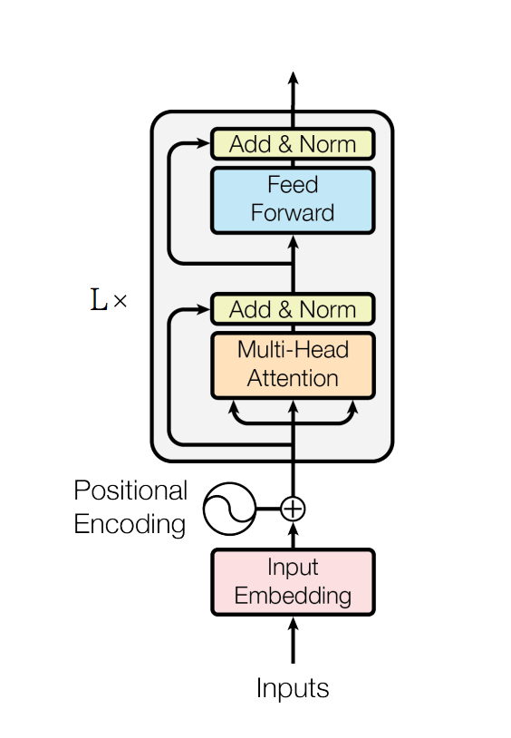
The input to the BERT model is a sequence of word tokens. These are first embedded into vectors of size E (BERT uses WordPiece embeddings with a vocabulary size V of 30,000) and then passed through the neural network. The encoder segment of the BERT model is shown in Figure 3. It primarily consists of a multi-head attention segment which computes self-attention over the inputs (the number of self-attention heads is denoted by A) and a position-wise feed-forward network (after each substep, residuals are added back and the output is normalized); the intermediate output of the encoder has a size of H (the hidden size). BERT essentially contains L such encoder blocks in its architecture.
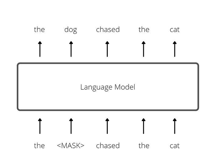
Pre-training the BERT model involves two tasks: (1) Masked Language Modeling (MLM) and (2) Next Sentence Prediction (NSP). In the first step (MLM), 15% of the words in the input sequence are replaced with the <MASK> token and the model attempts to predict the masked words based on the (bidirectional) context provided by the non-masked words (see example in Figure 4). The cross-entropy loss is used for this task (only masked words are counted).
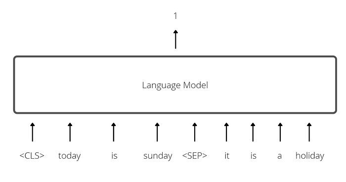
The second task (NSP) ensures that the model learns sentence-level information. Here, the input consists of token sequences of two sentences A & B with a <SEP> token in the middle. The model must then predict whether sentence B naturally follows sentence A (see example in Figure 5); positive examples for this task can be generated by passing two consecutive sentences from the training corpus to the model, while negative examples involve selecting two random sentences from different parts of the text and stitching them together.
Scalability Issue w/ BERT
____
Now that we have a basic understanding of the architecture of BERT, let’s consider the computational requirements for the pre-training step.
BERT comes in two flavors, each with a different set of hyperparameters:
(1) BERT base: number of encoder blocks (L) = 12, embedding size (E) = hidden size (H) = 768, number of self-attention heads (A) = 12. Total number of parameters = 110M
(2) BERT large: number of encoder blocks (L) = 24, embedding size (E) = hidden size (H) = 1024, number of self-attention heads (A) = 16. Total number of parameters = 340M
Both models have a vocabulary size (V) of 30,000.
Based on the above, the number of parameters for a model increases with
A) more encoder blocks L
B) longer WordPiece embeddings E (and a larger hidden size H)
C) larger vocabulary size V
(Note: The number of self-attention heads is typically set to be H / 64, so it is accounted for in the hidden size.)
To obtain a better language understanding for NLP tasks, it is logical that we would need our vocabulary to be as large as possible (so that our model understands more types of words) and the embeddings for each word should also be longer (to get a more accurate representation of their semantic context). Additionally, we know that deeper neural networks typically provide better predictions than shallow models. It is easy to see how the number of parameters in a BERT model could explode as we try to increase any (or all) of these. Therefore, we need a better approach for scaling LLMs.
ALBERT: A Lite BERT
____
In the paper ALBERT: A Lite BERT for Self-supervised Learning of Language Representations, authors Lan et al. have proposed ALBERT, a modified version of the BERT architecture with significantly fewer parameters (thereby allowing the model to scale easier) [Lan et al.]1. This modified model incorporates 3 key changes to the original BERT architecture that solve (to some extent) the limitations discussed earlier. The following sections explain each one in more detail.
Factorized Embedding Parameterization
One of the problems with BERT is that we have a V x H embedding matrix in the first layer of the neural network (mapping the one-hot vector of the input word to its hidden state representation) — i.e. the number of parameters in the first layer is O(V x H). So if we want to make the vocabulary larger, the size of the hidden state also increases.
The problem here is that, in the original BERT model, authors have tied the embedding size E to the hidden size H. However, Lan et al. argue that this is not the right approach as the WordPiece embeddings are meant to learn context-independent representations while the hidden-layer embeddings are meant to learn context-dependent representations — both of which are independent.

To resolve this issue, Lan et al. propose that the V x H embedding matrix be decomposed into two smaller matrices of size V x E and E x H (as shown in Figure 6). Doing this two-step embedding (input one-hot vector to WordPiece embedding and WordPiece embedding to hidden state representation) allows us to increase the vocabulary size V without increasing the number of parameters in the hidden layer. Therefore, this approach reduces the number of parameters in the embedding matrix from O (V x H) to O(V x E + E x H) which is significantly lesser when H >> E (which is ideal since we may want to have larger hidden layers to get better context-dependent representations, but without changing our WordPiece embeddings).
Cross-Layer Parameter Sharing
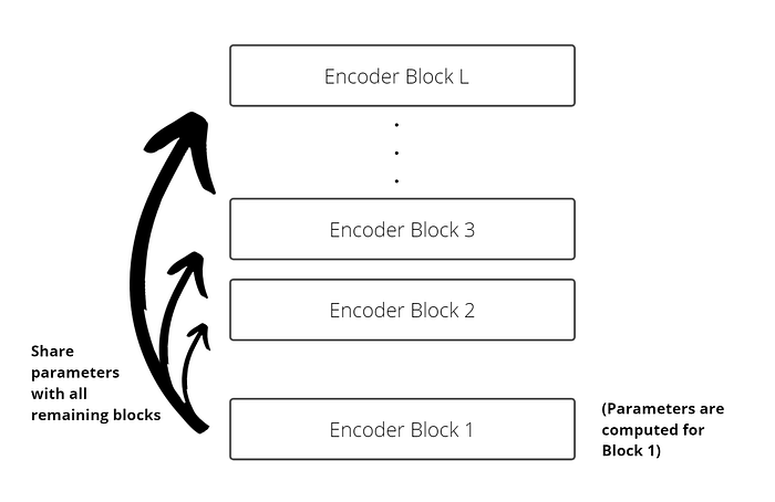
Another way ALBERT reduces the number of parameters is by sharing parameters across all encoder blocks (see Figure 7) — i.e. the parameters are computed for the first encoder layer and the same parameters are then used for all remaining layers. Doing this, the number of parameters no longer depends on the depth of the neural network L, which allows us to train deeper models.
Note: In the ALBERT implementation, all parameters are shared across encoder layers. Alternative strategies may involve only sharing the attention parameters or the parameters of the feed-forward network.
Inter-sentence Coherence Loss
A final change to the BERT model is the addition of a new type of loss to the pre-training process. Unlike the previous modifications, this is not meant to reduce the number of parameters but rather to improve the performance of the model.
The NSP (Next Sentence Prediction) loss in the original BERT model (described earlier) is a binary loss that predicts whether two sentences appear consecutively in the original text corpus. However, recent studies ([Yang et al. 2019]4; and [Liu et al. 2019]5) have shown that this NSP loss is unreliable and does not lead to better performance on downstream tasks. One possible explanation for this is that the NSP loss is too simplistic and yet tries to do both topic prediction (whether we are talking about the same thing in both sentences) and coherence prediction (whether the second sentence naturally follows from the first) in a single task.
Among the two, Lan et al. believed that topic prediction is easier to learn and also overlaps with what’s learned in the MLM loss (since predicting the right words in a sentence depends on knowing what topic the sentence is about). Accordingly, the authors focus on coherence prediction and replace the NSP loss with a Sentence-Order Prediction (SOP) loss. The difference here is that the positive examples are still consecutive sentences from the text corpus (like in NSP) but the negative examples are the same two sentences in reverse order (instead of two random sentences from different parts of the corpus) — this focuses the model on sentence cohesion and not topic prediction (we used random sentences earlier as sentences from different parts of the corpus would likely be about different topics; we do not want that here).
Performance of ALBERT vs BERT
____
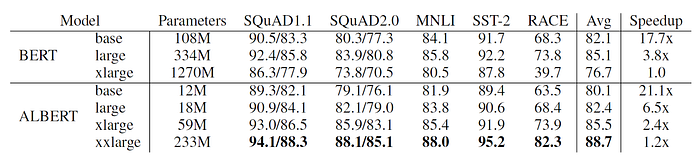
The primary benefit of ALBERT is that it has significantly fewer parameters as compared to the corresponding BERT model. Table 1 compares different versions of BERT and corresponding ALBERT implementations. As one can see, the ALBERT base model has 9x fewer parameters than its BERT counterpart, ALBERT large has 18.6x fewer parameters, and ALBERT xlarge has 21.5x fewer parameters. This clearly demonstrates that ALBERT scales way better than the original BERT implementation.

To compare the performance of ALBERT against BERT, the authors evaluated different versions of the two models during pre-training as well as on downstream tasks.
For the pre-training evaluation, the authors mimicked the testing environment of the original BERT model by using the same training corpuses and evaluated the MLM and sentence classification tasks on the SQuAD and RACE development sets. Table 2 summarizes the results of the pre-training evaluation. One can see that all the ALBERT variations are faster than their BERT counterparts. However, the average task score for the base and large models of ALBERT are lower than those of BERT. This means that at least an xlarge model is required for ALBERT to surpass BERT within 125k steps — increasing the number of training steps may provide a different result.
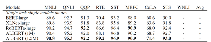
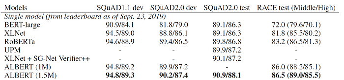
To evaluate performance of ALBERT on downstream tasks, the authors compared the performance of their best model configuration (ALBERT xxlarge) on the GLUE, SQuAD and RACE benchmarks. Tables 3 & 4 show how ALBERT compared against other state-of-the-art models like BERT, XLNet, RoBERTa and others. Once again, we see that ALBERT (trained at 1M steps and 1.5M steps) achieves better performance than all other models.
Conclusion
____
In this article, we have provided a high-level summary of the ALBERT model developed by Lan et al. We have discussed the modifications in ALBERT over the original BERT model and how these lead to significantly fewer parameters (allowing us to scale models easier) and better performance on downstream tasks. Experimental results from the paper have also been briefly mentioned to provide a numerical backing to the hypothesized benefits of ALBERT. Interested readers may read the original paper to get a more detailed analysis of this implementation.
References
____
[1] Lan, Zhenzhong et al. “ALBERT: A Lite BERT for Self-supervised Learning of Language Representations”. International Conference on Learning Representations. N.p., 2020. Web.
[2] Devlin, Jacob et al. “BERT: Pre-training of Deep Bidirectional Transformers for Language Understanding”. arXiv [cs.CL] 2019. Web.
[3] Vaswani, Ashish et al. “Attention Is All You Need”. arXiv [cs.CL] 2017. Web.
[4] Zhilin Yang, Zihang Dai, Yiming Yang, Jaime Carbonell, Ruslan Salakhutdinov, and Quoc V Le. XLNet: Generalized autoregressive pre-training for language understanding. arXiv preprint arXiv:1906.08237, 2019.